Intro

One of the ultimate goals of sports analytics is to predict future outcomes based on some observed patterns in past events.

In this article, I will review the problem of predicting the percentage of games won by a team in (European) football in one of the most popular leagues – the English Premier League (EPL).

I’ll explore a metric called Pythagorean Expectation that originated in baseball but happens to apply to football as well.

This article is based on the materials in the Coursera course – Foundations of Sports Analytics: Data, Representation, and Models in Sports.

What is Pythagorean Expectation, and How is it Helpful?

Pythagorean Expectation (or Pythagorean Winning Percentage) was devised by Bill James – a famous statistician who devoted his work to baseball history and statistics.

It deals with predicting how many games a team should have won based on the number of runs it has scored and allowed (in football, instead of runs, we will use the goals scored and goals received).

Having such a win percentage expectation allows you to potentially forecast future winning/losing streaks if a team is currently under/over performing.

Let’s say you have the data for all of the team’s games in the first half of the season. How can you use that data to predict the winning percentage of the second half of the season?

One approach would be to get the win percentage from the first half and expect the same win percentage for the second half.

This sounds reasonable. However, Bill has shown (and we will confirm the same for football) that you will be more successful if you base your predictive analysis on the runs (goals in football) using the following formula:

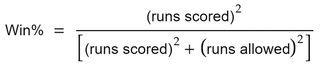
For football, the equation looks like so:

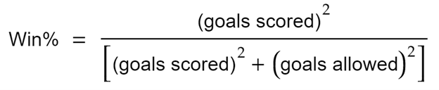
The formula is quite simple.

Pythagorean Win Percentage is not the most advanced and accurate measure, but it can give many insights and has proven to have decent predictive power. Also, it can be used as a baseline for a more sophisticated model.

For the rest of this article, I will explore a football dataset for the English Premier League. By the end, you will see for yourself that the Pythagorean Expectation applies to football as well.

The Notebook

You can access(and execute) the complete source code in Google Colabs here.

I have intentionally not copied here most of the code dealing with the data preparation as it adds distractions to the main takeaways. I encourage you to explore the implementation details on your own.

The more exciting part is the resulting analysis and graphics that I will focus on.

Prepare the Data

For this demo, I’ve used the EPL data for the 2017-2018 season that you can find here.

Let’s have a quick look at the dataset (after simplifying it):

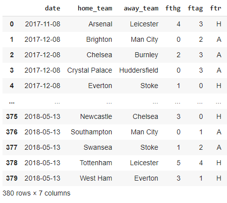
There are 380 rows (games) in an EPL season. For every game, we have the date, the home team, the away team, the full-time home team goals(fthg), the full-time away team goals(ftag), and the full-time result(ftr).

Remember, the final goal is to examine the forecasting power of Pythagorean Expectation for the second part of the season based on the first half.

That’s why our first step is to split the games into two – the ones in the first half of the season (played in 2017) and the ones in the second half (played in 2018).

Winning Percentages

Next, for each half, we calculate the win percentage for every team.

So, for the first half, we get the following output:

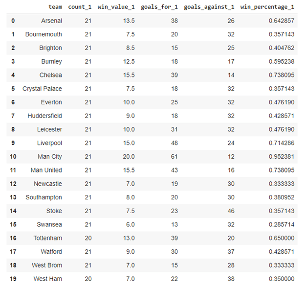
The last column holds the win percentage. The _1 suffix in the column names indicates that this value is for the first half of the season.

The second half data looks like so:

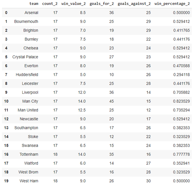
You may be wondering how the win percentage is exactly calculated.

Basically, if a team has won a game, this adds 1 to its total wins. If the team lost, it doesn’t add anything. If the game was a draw – both teams take 0.5 to their win value. Here’s the function that implements the described logic:

def get_win_value(team):
  if team['ftr'] == 'H' and team['home'] == 1:
    return 1
  if team ['ftr'] == 'A' and team['home'] == 0:
    return 1
  if team ['ftr'] == 'D':
    return 0.5
  return 0

In the end, the total win value for each team is divided by the number of games the team has played, and that’s the final winning percentage.

Quick example – a team with a win, a draw, and a loss will have a total win percentage of 0.5, resulting from the expression: (1 + 0.5 + 0)/3

Pythagorean Expectations

Now that we have the win percentages, let’s calculate the Pythagorean Expectations, again for the first and second halves of the season.

We’ll use the function below for each row in the dataset:

def calc_pyth_exp(goals_for, goals_agains):
  return goals_for**2 / (goals_for**2 + goals_agains**2)

Here’s the result for the first half of the season – see the last column:

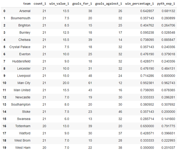
Let’s plot a simple linear regression between win_percentage_1 and pyth_exp_1:

You can clearly see a quite strong linear correlation between the variables.

Now, let’s calculate the Pythagorean Expectation for the second half of the season as well:

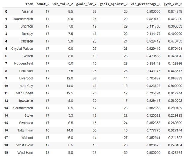
And plot a similar regression.

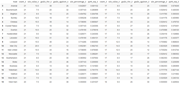
Now, we’d like to take a step further and see how the Pythagorean Expectation from the first half of the season correlates to the win percentage of the second half.

For that, let’s start by merging the two datasets so that we can easily analyze relationships between variables from the first and second half:

The Forecasting Power of Pythagorean Winning Percentage

First, let’s plot a linear regression between win_percentage_1 and win_percentage_2.

There is clearly some linear correlation, although not super strong. We’ll explore this numerically a little later.

Next, let’s create a similar plot but use pyth_exp_1 as an independent variable.

This plot looks very similar to the previous one.

Visually, we can’t judge whether win_percentage_1 or pyth_exp_1 is a better predictor for win_percentage_2.

So, let’s review the exact correlation coefficients between all the variables of interest in the dataset:

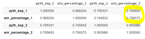
From this table, you can see that there’s a stronger correlation between pyth_exp_1 and win_percentage_2 (0.796) than win_percentage_1 and win_percentage_2 (0.757).

This proves that the Pythagorean Expectation is has a stronger forecasting power than the win percentage.

This outcome is precisely what Bill James analyzed and proved for baseball. Not surprisingly, it holds for football as well.

Summary

In this article, I explored a metric called Pythagorean Expectation that strongly relates to the winning percentage of a specific team. This can be helpful when forecasting winning/losing streaks for a team that is under/overperforming.

We also confirmed the initial assumption that the Pythagorean Expectation measure has a more substantial predictive power than the past winning percentage itself.

In the next article, I will explore the effect money has on modern football. Concretely, I will build a Machine Learning model for predicting games outcome based solely on Transfermark data.

See you next time!

Resources

1. Foundations of Sports Analytics: Data, Representation, and Models in Sports